• select an area of ​​cells;
• use the “AutoSum” button;
• create formula simple addition;
• using the function.

How to calculate the amount in a column in Excel

Calculate the sum by selecting an area of ​​cells

Firstly, you can find out the sum of any cells with values ​​by simply selecting the cells you need with the left mouse button:

By selecting the cells with numbers, Excel displays the sum of the values ​​in the range you selected in the lower right corner.

In order to select cells that are not adjacent, you should hold down CTRL key and select cells with the left mouse button.

How to calculate the sum in a column using the simple addition formula

Perhaps the simplest and most primitive way of summing data in a column is the simple addition formula. To summarize data:

• left-click on the cell in which you want to get the addition result;
• enter the formula:

In the formula above, indicate the numbers of the cells that you want to sum:

How to calculate the amount in a column using the “AutoSum” button

If you want to calculate the sum of numbers in a column and leave this result in the table, then perhaps the easiest way is to use the “AutoSum” function. It will automatically determine the range of cells required for summation and save the result in the table.

To count the numbers in a column using AutoSum, do the following:

• Click on the first empty cell in the column under the values ​​you want to sum:

• Select the “AutoSum” icon on the toolbar:

• After pressing the button, the system will automatically select the range for summation. If the system has chosen the range incorrectly, you can correct it simply by changing the formula:

• Once you are sure that the range of values ​​for the amount is selected correctly, simply press the Enter key and the system will calculate the amount in the column:

How to calculate the amount in a column using the SUM function in Excel

You can add the values ​​in a column using the function. Most often, a formula is used to create the sum of individual cells in a column or when the cell containing the sum does not need to be located directly below the data column. To calculate the amount using the function, follow these steps:

• Select the cell with the left mouse button and enter the “ ” function, specifying the required range of cells:

• press the “Enter” button and the function will calculate the amount in the specified range.

How to calculate the amount in a column in Excel using a table

To calculate the sum of a data column, you can format the data as a table. For this:

• Select a range of cells with data and convert them into a table using the “Format as Table” button on the toolbar:

• Once your data is presented in table format, on the “Design” tab in the toolbar, select “Total Row” to add the sum of the columns below the table:

How to calculate the sum in several columns in Excel at the same time

In this lesson we will not look at how to calculate a sum in Excel using the addition operator, autosum and other tools. Today we will look at just two functions: SUM And SUMIF. I hasten to please you, their functionality is enough to solve almost everything possible questions summation in Excel.

SUM function - simple summation of cells in Excel

Function SUM calculates the sum of all its arguments. It is the most commonly used function in Excel. For example, we need to add the values ​​in three cells. We can of course use regular operator summation:

But we can also use the function SUM and write the formula as follows:

Since the function SUM supports work not only with separate cells, but also entire ranges, then the above formula can be modified:

The true power of the feature SUM opens when folded a large number of cells in Excel. The example below requires summing 12 values. Function SUM allows you to do this with a few clicks of the mouse, but if you use the addition operator, it will take a long time.

In the following example, the function SUM adds up the entire column A, which is 1048576 values:

The following formula calculates the sum of all cells contained in a worksheet Sheet1. To this formula did not cause a cyclic error, it must be used on another worker Excel sheet(different from Sheet1).

Function SUM can take up to 255 arguments and sum several non-adjacent ranges or cells at once:

If the summed values ​​contain text, then the function SUM ignores them, i.e. does not include in the calculation:

If text values try to add using the summation operator, the formula will return an error:

Function SUM is quite universal and allows you to use as arguments not only references to cells and ranges, but also various mathematical operators and even other Excel functions:

SUMIF – conditional sum in Excel

For example, the following formula is summed only positive numbers range A1:A10. Note that the condition is enclosed in double quotes.

You can use the cell value as a condition. In this case, changing the condition will change the result:

We change the condition, and the result changes:

Conditions can be combined using the concatenation operator. In the example below, the formula will return the sum of the values ​​that are greater than the value in cell B1.

In all the examples given earlier, we summed and checked the condition over the same range. But what if you need to sum one range and check the condition differently?

In this case the function SUMIF has a third optional argument, which is responsible for the range that needs to be summed. Those. the function checks the condition using the first argument, and the third is subject to summation.

In the following example, we will add up the total cost of all fruits sold. To do this, we use the following formula:

Clicking Enter we get the result:

If one condition is not enough for you, then you can always use the function SUMIFS, which allows you to perform conditional summation in Excel based on several criteria.

Summation is one of the main actions that the user performs in Microsoft Excel. Functions SUM And SUMIF created to make this task easier and give users the most handy tool. I hope this lesson helped you learn basic functions summation in Excel, and now you can freely apply this knowledge in practice. Good luck to you and success in learning Excel!

Tabular Excel processor – perfect solution for processing various types of data. With its help, you can quickly make calculations with regularly changing data. However, Excel is a rather complex program and therefore many users do not even begin to learn it.

In this article we will talk about how to calculate the amount in Excel. We hope this material will help you become familiar with Excel and learn how to use its basic functions.

Also, the “Auto sum” button is duplicated on the “Formula” tab.

After you highlight a data column and click the Auto Sum button, Excel will automatically generate a formula to calculate the column's sum and insert it into the cell immediately below the data column.

If this arrangement of the column sum does not suit you, then you can specify where you want to place the sum. To do this, you need to select the cell suitable for the sum, click on the “AutoSum” button, and then select the column with the data with the mouse and press the Enter key on the keyboard.

In this case, the column sum will not be located under the data column, but in the table cell you selected.

How to calculate the sum of specific cells in Excel

If you need to calculate the sum of certain cells in Excel, then this can also be done using the Auto Sum function. To do this, you need to select the table cell in which you want to place the amount with the mouse, click on the “Auto Sum” button and select the desired cells while holding down the CTRL key on the keyboard. Once the desired cells are selected, press the Enter key on your keyboard and the amount will be placed in the table cell you selected.

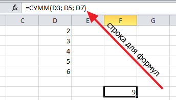
In addition, you can enter a formula to calculate the sum of certain cells manually. To do this, place the cursor where the amount should be, and then enter the formula in the format: =SUM(D3; D5; D7). Where instead of D3, D5 and D7 are the addresses of the cells you need. Please note that cell addresses are entered separated by commas; a comma is not needed after the last cell. After entering the formula, press the Eneter key and the sum will appear in the cell you selected.

If the formula needs to be edited, for example, you need to change the cell addresses, then to do this you need to select the cell with the amount and change the formula in the formula bar.

How to quickly view the amount in Excel

If you need to quickly see what the total will be if you add it up specific cells, and you don’t need to display the sum value in the table, then you can simply select the cells and look down Excel windows. There you can find information about the sum of the selected cells.

The number of selected cells and their average value will also be indicated there.

Hello!

Many who don’t use Excel don’t even imagine what opportunities this program provides! Just think: fold in automatic mode values ​​from one formula to another, look for required lines in the text, fold according to condition, etc. - in general, essentially a mini-programming language for solving “narrow” problems (to be honest, I myself for a long time I didn’t consider Excel as a program, and almost didn’t use it)...

In this article I want to show several examples of how you can quickly solve everyday problems. office tasks: add something, subtract something, calculate a sum (including with a condition), substitute values ​​from one table into another, etc. That is, this article will be something like a mini guide on learning what you need for work (more precisely, to start using Excel and feel the full power of this product!).

It is possible that if I had read a similar article 15-17 years ago, I myself would have been much more started faster use Excel (and would save a lot of my time solving "simple" (note: as I understand it now) tasks)...

Note: All screenshots below are from Excel programs 2016 (as the newest to date).

Many novice users, after launch Excel- they ask one strange question: “well, where is the table?” Meanwhile, all the cells that you see after starting the program are one big table!

Now to the main thing: any cell can contain text, some number, or a formula. For example, the screenshot below shows one illustrative example:

• left: cell (A1) contains the prime number "6". Please note that when you select this cell, the formula bar (Fx) simply shows the number "6".
• on the right: in cell (C1) there is also a simple number “6”, but if you select this cell, you will see the formula "=3+3" - this is an important feature in Excel!

Just a number (on the left) and a calculated formula (on the right)

The point is that Excel can calculate like a calculator if you select some cell and then write a formula, for example "=3+5+8" (without quotes). You don’t need to write the result - Excel will calculate it itself and display it in the cell (as in cell C1 in the example above)!

But you can write in formulas and add not just numbers, but also numbers that have already been calculated in other cells. In the screenshot below, in cells A1 and B1 there are numbers 5 and 6, respectively. In cell D1 I want to get their sum - you can write the formula in two ways:

• first: “=5+6” (not very convenient, imagine that in cell A1 - our number is also calculated according to some other formula and it changes. You won’t substitute a new number instead of 5 every time?!);
• the second: “=A1+B1” - but this is the ideal option, we simply add the values ​​of cells A1 and B1 (despite even what numbers are in them!)

Adding cells that already contain numbers

Spreading a formula to other cells

In the example above, we added the two numbers in column A and B in the first row. But we have 6 lines, and most often in real problems you need to add numbers in each line! To do this, you can:

1. in line 2 write the formula "=A2+B2", in line 3 - "=A3+B3", etc. (this is long and tedious, this option is never used);
2. select cell D1 (which already has a formula), then move the mouse pointer to the right corner of the cell so that a black cross appears (see screenshot below). Then pinch left button and stretch the formula to the entire column. Convenient and fast! (Note: you can also use the combinations Ctrl+C and Ctrl+V for formulas (copy and paste, respectively)).

By the way, pay attention to the fact that Excel itself inserted formulas into each line. That is, if you now select a cell, say D2, you will see the formula "=A2+B2" (i.e. Excel automatically substitutes formulas and immediately produces the result) .

How to set a constant (a cell that will not change when you copy the formula)

Quite often it is required in formulas (when you copy them) that some value does not change. Let's say a simple task: convert prices in dollars to rubles. The value of the ruble is specified in one cell, in my example below it is G2.

Next, in cell E2, write the formula “=D2*G2” and get the result. But if we stretch the formula, as we did before, we won’t see the result in other lines, because Excel will put the formula “D3*G3” in line 3, “D4*G4” in line 4, etc. We need G2 to remain G2 everywhere...

To do this, simply change cell E2 - the formula will look like "=D2*$G$2". Those. dollar sign $ - allows you to specify a cell that will not change when you copy the formula (i.e. we get a constant, example below)...

How to calculate the amount (formulas SUM and SUMIFS)

You can, of course, compose formulas in manual mode, typing "=A1+B1+C1" etc. But Excel has faster and more convenient tools.

One of the most simple ways to add all selected cells is to use the option autosums (Excel will write the formula itself and insert it into the cell).

1. First, select the cells (see screenshot below);
2. Next, open the “Formulas” section;
3. The next step is to click the "AutoSum" button. The result of the addition will appear under the cells you selected;
4. if you select the cell with the result (in my case it is the cell E8) - then you will see the formula "=SUM(E2:E7)" .
5. thus, writing the formula "=SUM(xx)", where instead xx put (or select) any cells, you can read a wide variety of ranges of cells, columns, rows...

Quite often when working, you need not just the sum of the entire column, but the sum certain lines(i.e. selectively). Suppose simple task: you need to get the amount of profit from some worker (exaggerated, of course, but the example is more than real).

I will use only 7 rows in my table (for clarity), but a real table can be much larger. Suppose we need to calculate all the profits that “Sasha” made. What the formula will look like:

1. "=SUMIFS(F2:F7 ;A2:A7 ;"Sasha") " - (note: pay attention to the quotation marks for the condition - they should be as in the screenshot below, and not as I have written on my blog now). Also note that Excel, when entering the beginning of a formula (for example, “SUM..."), itself prompts and substitutes possible options- and there are hundreds of formulas in Excel!;
2. F2:F7 is the range over which the numbers from the cells will be added (summed);
3. A2:A7 is the column against which our condition will be checked;
4. “Sasha” is a condition, those rows in which “Sasha” is in column A will be added (pay attention to the indicative screenshot below).

Note: there can be several conditions and they can be checked using different columns.

How to count the number of lines (with one, two or more conditions)

A fairly typical task: to count not the sum in the cells, but the number of rows that satisfy some condition. Well, for example, how many times the name “Sasha” appears in the table below (see screenshot). Obviously 2 times (but this is because the table is too small and taken as clear example). How to calculate this with a formula? Formula:

"=COUNTIF(A2:A7,A2)" - Where:

• A2:A7- the range in which rows will be checked and counted;
• A2- a condition is set (note that you could write a condition like “Sasha”, or you can simply specify a cell).

The result is shown on the right side of the screen below.

Now imagine a more advanced task: you need to count the lines where the name “Sasha” appears, and where in the AND column the number “6” will appear. Looking ahead, I will say that there is only one such line (screenshot with an example below).

The formula will look like:

=COUNTIFS(A2:A7 ;A2 ;B2:B7 ;"6") (note: pay attention to the quotation marks - they should be like in the screenshot below, and not like mine), Where:

A2:A7 ;A2- the first range and search condition (similar to the example above);

B2:B7 ;"6"- the second range and search condition (note that the condition can be set in different ways: either by specifying a cell, or simply by text/number written in quotes).

How to calculate the percentage of the amount

This is also a fairly common question that I often encounter. In general, as far as I can imagine, it arises most often - due to the fact that people are confused and do not know what they are looking for a percentage of (and in general, they do not understand the topic of percentages well (although I myself am not a great mathematician, and still ... )).

The simplest way, in which it is simply impossible to get confused, is to use the “square” rule, or proportions. The whole point is shown in the screenshot below: if you have total amount, let’s say in my example this number is 3060 - cell F8 (i.e. this is 100% profit, and some part of it was made by “Sasha”, you need to find which one...).

In proportion, the formula will look like this: =F10*G8/F8(i.e. cross by cross: first we multiply two known numbers diagonally, and then divide by the remaining third number). In principle, using this rule, it is almost impossible to get confused in percentages.

Actually, this is where I conclude this article. I’m not afraid to say that having mastered everything that is written above (and only “five” formulas are given here), you will then be able to independently learn Excel, leaf through the help, watch, experiment, and analyze. I’ll say even more, everything that I described above will cover many tasks, and will allow you to solve the most common ones, which you often puzzle over (if you don’t know Excel capabilities), and you don’t know how to do it faster...

Date: February 29, 2016 Category:

Hello friends. Today we are learning how to count cells in Excel. These functions solve a wide range of problems for representatives of many professions. By performing intermediate calculations, they become the basis for automating your calculations. I know many managers who use counting functions to work with their impressive range of products.

If you just need to know the number of values ​​without using them in calculations, it is convenient to look at the data in the status bar:

Number of values ​​in the status bar

You can select the indicators displayed in the line by clicking on it right click mice.

Customizing the Status Bar

If you need to use the number of values ​​in further calculations, use the functions described below. For convenience of notation, we will assume that the data array for which the count is being made is . In your formulas, you can use the desired data range instead of the name.

How to count the number of cells in Excel

To count the number of cells in Excel, there are two functions:

1. LINE(array) – counts the number of lines in the selected range, regardless of what its cells are filled with. The formula gives results only for a rectangular array of adjacent cells, otherwise ;

Counting the number of lines

1. NUMCOLUMN(array)– similar to the previous one, but counts the number of array columns

Excel doesn't have a function to determine the number of cells in an array, but it can be easily calculated by multiplying the number of rows by the number of columns: =NUMROW(array)*NUMBERCOLUMN(array).

How to count empty cells in Excel

We count empty cells

The function considers a cell empty if there is nothing written in it, or the formula inside it returns an empty string.

How to count the number of values ​​and numbers in Excel

Counting numerical values

If we need to determine the number of cells containing values, we use the function COUNTA(value1,value2,…). Unlike the previous function, it will count not only numbers, but also any combination of symbols. If the cell is not empty, it will be counted. If there is a formula in the cell that returns zero or an empty string, the function will also include it in its result.

Count non-empty cells

How to count cells with a condition in Microsoft Excel

• Array – a range of cells among which the count is performed. You can only specify a rectangular range of adjacent cells;
• Criterion – the condition by which selection occurs. Write text conditions and numeric conditions with comparison signs in quotation marks. We write equal numbers without quotes. For example:
  • “>0” – count cells with numbers greater than zero
  • “Excel” – count cells containing the word “Excel”
  • 12 – counting cells with the number 12

Counting cells with condition

If you need to take into account several conditions, use the function COUNTIFS(array1,criteria1,[array2],[criteria1]…). The function can contain up to 127 array-criteria pairs.

If you use different arrays in one such function, they should all contain the same number of rows and columns.

Counting values ​​based on multiple conditions

How to determine the most common number

To find the number that occurs most often in an array, there is a function in Excel MODE(number1;number2;…). The result of its execution will be the same number that occurs most often. To determine their number, you can use a combination of summation formulas and array formulas.

If there are several such numbers, the one that appears earlier in the list will be displayed. The function only works with numeric data.

Frequently occurring number

This is, perhaps, the entire list of functions that I want to present to you as part of this post. They are quite enough to solve the most popular cell counting problems. Combine them with other features (eg) to get maximum results.

In the next article we will study. Go read it, even if you are sure you know everything about it. I think there will be something there just for you!